Arrays and Structures (2)

Polynomials

The Abstract Data Type

이번 포스트에서는 지난 포스트에서 배운 자료구조를 토대로 응용하는 방법을 알아보겠습니다. 가장 먼저 다뤄볼 문제는 다항식(Polynomial)입니다. 다항식은 고등학교 때 지겹게 다뤄보셨을테니 간단하게만 설명하고 넘어가겠습니다. 다항식은 $ax^b$와 같은 형태를 가지고 있는 항들의 합으로 나타나는 식입니다. 여기서 $a$는 계수(Coefficient)라고 부르고, $x$는 변수(Variable), $b$는 차수(Exponent)라고 부릅니다. 다항식의 예로는 $5x^2+2x+3$ 같은 식이 있습니다.

다항식의 추상 데이터 타입(ADT)은 다음과 같이 정의됩니다.

ADT Polynomial is
    Object : p(x)=a_1 * x^{e_1} + ... + a_n * x^{e_n}; a set of ordered pairs of <a_i, e_i> where a_i in Coefficients and e_i in Exponents are integers >= 0  
    Functions :
        for all poly, poly1, poly2 ∈ Polynomial, coef ∈ Coefficients, expon ∈ Exponents

        Polynomial Zero()                            ::= return the polynomial p(x) = 0
        Boolean IsZero(poly)                         ::= if (poly) return FALSE
                                                         else return TRUE
        Coefficients Coef(poly,expon)                ::= if (expon ∈ poly) return its coefficient
                                                         else return zero
        Exponent LeadExp(poly)                       ::= return the largest exponen in poly
        Polynomial Attach(poly,coef,expon)           ::= if (expon ∈ poly) return error
                                                         else return the polynomial poly with the term <coef,expon> inserted
        Polynomial Remove(poly,expon)                ::= if (expon ∈ poly) the polynomial poly with the term whose exponent is expon deleted
                                                         else return error
        Polynomial SingleMult(poly,coef,expon)       ::= return the polynomial poly * coef * x^{expon}
        Polynomial Add(poly1,poly2)                  ::= return the polynomial poly1 + poly2
        Polynomial Mult(poly1,poly2)                 ::= return the polynomial poly1 * poly2
end Polynomial

Polynomial Representation

이제 다항식을 프로그램에서 어떻게 표현할지 고민해보겠습니다. 먼저, 다항식은 기본적으로 내림차순으로 정렬되어 있다고 가정합니다. 다항식이 내림차순으로 정렬되어 있다는 것은 가장 높은 차수를 가진 항부터 차수 순서대로 정렬되어 있다는 뜻입니다. 예시를 들었던 다항식 $5x^2+2x+3$이 내림차순으로 정렬된 다항식의 예입니다.

이 경우 가장 먼저 생각해볼 수 있는 방법은 각 항의 계수를 배열에 저장하는 것입니다. 예를 들어, coef[10]이라는 배열이 있다면 coef[0]에는 상수항, coef[1]에는 1차항의 계수, coef[2]에는 2차항의 계수, … 와 같이 설계하는 것입니다. 어차피 $x$는 고정이니 고려할 필요가 없고, 배열의 index가 곧 차수가 됩니다. 이렇게 설계한 Polynomial 구조체는 다음과 같이 선언할 수 있습니다.

#define MAX_DEGREE 101
 typedef struct {
	 int degree;
	 float coef[MAX_DEGREE];
 } Polynomial;

이 경우 구현이 매우 간단하다는 장점이 있지만, 그에 못지 않은 단점도 많습니다. 우선 이 방법을 사용하기 위해서는 프로그램에 사용되는 다항식의 차수가 얼마나 높은지 미리 알고 있어야 합니다. 미리 알고 있다고 해도, 다루는 다항식에 따라 저장 공간의 낭비가 굉장히 발생하기 쉬운 구조입니다.

예를 들어, 위와 같이 100차항을 다룰 수 있는 구조체를 선언했지만 실제로 3~4차 정도의 간단한 다항식만 다루는 경우에는 실수형 배열 coef의 90% 이상이 낭비되고 맙니다. 게다가 실제로 높은 차수를 사용하더라도, $2x^{100} + 1$과 같이 다항식이 Sparse한 경우에도 많은 공간이 낭비됩니다. 그렇기 때문에 저장 공간의 낭비를 줄이기 위해, 다음과 같은 방법으로 수정해보겠습니다.

#define MAX_TERMS 100
typedef struct {
	float coef;
	int expon;
} polynomial;
polynomial terms[MAX_TERMS];
int avail = 0;

이 방법은 아까보다 조금 복잡한 방법이기 때문에 설명이 필요할 것 같습니다. 먼저 두 다항식 $A(x) = 2x^{100} + 1$과 $B(x) = x^4 + 10x^3 + 3x^2 + 1$이 주어졌다고 가정합니다. 그 두 다항식을 이 구조체 배열에 저장한다면 다음과 같이 구조가 됩니다.

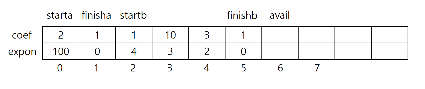
여러 개의 다항식을 하나의 2차원 배열에 저정하기 때문에 이를 구별하기 위해 여러 변수를 사용합니다. starta, startb는 다항식 $A(x)$, $B(x)$의 시작 index이고, finisha, finishb는 끝 index입니다. avail은 배열에서 사용하고 남아 있는 부분의 시작 index입니다. 만약 새로운 다항식 $C(x)$를 추가하고 싶다면 startc를 현재 avail과 같은 값으로 선언하고, 다항식 끝 index를 finishc로 선언, 그 다음 index를 avail로 선언하시면 됩니다.

Polynomial Addition

이제 두 개의 다항식을 더하는 함수를 만들어보겠습니다. 두 개의 다항식을 더한 새로운 다항식을 만든 후, 그 다항식도 terms에 저장하는 프로그램을 만들면 다음과 같습니다.

Program 2.6: Function to add two polynomials

void padd(int starta, int finisha, int startb, int finishb, int* startd, int* finishd) {
	/* add A(x) and B(x) to obtain D(x) */
	float coefficient;
	*startd = avail;
	while (starta <= finisha && startb <= finishb)
		switch (COMPARE(terms[starta].expon, terms[startb].expon)) {
		case -1: /* a expon < b expon */
			attach(terms[startb].coef, terms[startb].expon);
			startb++;
			break;
		case 0: /* equal exponents */
			coefficient = terms[starta].coef + terms[startb].coef;
			if (coefficient)
				attach(coefficient, terms[starta].expon);
			starta++; startb++;
			break;
		case 1: /* a expon > b expon */
			attach(terms[starta].coef, terms[starta].expon);
			starta++;
		}
	/* add in remaining terms of A(x) */
	for (; starta <= finisha; starta++)
		attach(terms[starta].coef, terms[starta].expon);
	/* add in remaining terms of B(x) */
	for (; startb <= finishb; startb++)
		attach(terms[startb].coef, terms[startb].expon);
	*finishd = avail - 1;
}

padd 함수는 두 다항식을 더한 후 terms에 새로운 다항식을 이어붙이는 프로그램입니다. while 문을 반복하는 동안 다항식 A와 B의 차수를 비교하면서 A의 차수가 더 큰 항인 경우 A의 계수를, B의 차수가 더 큰 경우에는 B의 계수를 입력하며 차수가 같은 경우에는 두 항의 계수를 더하는 방식입니다.

함수 padd는 두 다항식 A와 B 전체를 탐색하기 때문에 $O(m+n)$의 시간 복잡도를 갖습니다. (단, 다항식 A의 항 개수는 m, 다항식 B의 항 개수는 n입니다)

padd의 함수를 보시면 attach라는 함수가 보이는데, 이것은 새로운 항을 추가하는 함수입니다. attach 함수는 다음과 같이 구현할 수 있습니다.

Program 2.7: Function to add a new term

void attach(float coefficient, int exponent) {
	/* add a new term to the polynomial */
	if (avail >= MAX_TERMS) {
		fprintf(stderr, "Too many terms in the polynomial\n");
		exit(EXIT_FAILURE);
	}
	terms[avail].coef = coefficient;
	terms[avail++].expon = exponent;
}

padd 함수, attach 함수에 main 함수를 포함하여 전체 프로그램을 구현하면 다음과 같습니다.

#include <stdio.h>
#include <stdlib.h>

#define COMPARE(x, y) (((x) < (y)) ? -1 : ((x) == (y)) ? 0 : 1)

#define MAX_TERMS 100
typedef struct {
	float coef;
	int expon;
} polynomial;

polynomial terms[MAX_TERMS];
int avail = 0;

void padd(int starta, int finisha, int startb, int finishb, int* startd, int* finishd);
void attach(float coefficient, int exponent);

int main() {
	int starta, finisha, startb, finishb, startd, finishd;

	/* input polynomial A */
	starta = 0;
	finisha = 1;
	terms[0].coef = 2;
	terms[0].expon = 1000;
	terms[1].coef = 1;
	terms[1].expon = 0;

	/* input polynomial B */
	startb = 2;
	finishb = 5;
	terms[2].coef = 1;
	terms[2].expon = 4;
	terms[3].coef = 10;
	terms[3].expon = 3;
	terms[4].coef = 3;
	terms[4].expon = 2;
	terms[5].coef = 1;
	terms[5].expon = 0;

	/* set the avail variable */
	avail = 6;
	
	/* calculate A(x) + B(x) = D(x) */
	padd(starta, finisha, startb, finishb, &startd, &finishd);

	for (int i = startd; i <= finishd; i++)
		printf("%f %d\n", terms[i].coef, terms[i].expon);

	return 0;
}

void padd(int starta, int finisha, int startb, int finishb, int* startd, int* finishd) {
	/* add A(x) and B(x) to obtain D(x) */
	float coefficient;
	*startd = avail;
	while (starta <= finisha && startb <= finishb)
		switch (COMPARE(terms[starta].expon, terms[startb].expon)) {
		case -1: /* a expon < b expon */
			attach(terms[startb].coef, terms[startb].expon);
			startb++;
			break;
		case 0: /* equal exponents */
			coefficient = terms[starta].coef + terms[startb].coef;
			if (coefficient)
				attach(coefficient, terms[starta].expon);
			starta++; startb++;
			break;
		case 1: /* a expon > b expon */
			attach(terms[starta].coef, terms[starta].expon);
			starta++;
		}
	/* add in remaining terms of A(x) */
	for (; starta <= finisha; starta++)
		attach(terms[starta].coef, terms[starta].expon);
	/* add in remaining terms of B(x) */
	for (; startb <= finishb; startb++)
		attach(terms[startb].coef, terms[startb].expon);
	*finishd = avail - 1;
}

void attach(float coefficient, int exponent) {
	/* add a new term to the polynomial */
	if (avail >= MAX_TERMS) {
		fprintf(stderr, "Too many terms in the polynomial\n");
		exit(EXIT_FAILURE);
	}
	terms[avail].coef = coefficient;
	terms[avail++].expon = exponent;
}

The Sparse Matrix

The Abstract Data Type

행렬 중 대부분의 값이 0인 행렬을 희소 행렬(Sparse Matrix)라고 부릅니다. 일반적으로 m * n 크기의 행렬을 저장할 때는 m * n 만큼의 2차원 배열을 이용하여 저장하지만, 희소 행렬의 경우 대다수의 원소가 0으로 구성되어 있기 때문에 이렇게 저장하면 공간이 많이 낭비되는 단점이 있습니다. 따라서 여기에서는 희소 행렬을 저장할 때 저장 공간을 절약하는 방법을 알아보겠습니다.

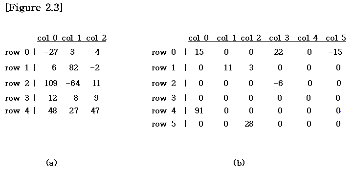
Figure 2.3에서 (a)가 일반적인 행렬, (b)가 희소 행렬의 예시입니다. 희소 행렬의 추상 데이터 타입은 다음과 같습니다.

ADT Sparse_Matrix is
    Object : a set of triples, <row, column, value>, where row and column are integers and from a unique combination, and value comes from the set item.
    Functions :
        for all a, b ∈ Sparse_Matrix, x ∈ item, i, j, max_col, max_row ∈ index

        Sparse_Matrix Create(max_row, max_col)    ::= return a Sparse_Matrix that can hold up to max_items = max_row×max_col and whose maximum row size is max_row and whose maximum column size is max_col
        Sparse_Matrix Transpose(a)                ::= return the matrix produced by interchanging the row and column value of every triple
        Sparse_Matrix Add(a, b)                   ::= if the dimension of a and b are the same
                                                      return the matrix produced by adding corresponding items, namely those with identical row and column values
                                                      else return error
        Sparse_Matrix Multiply(a, b)              ::= if number of columns in a equals number of rows in b
                                                      return the matrix d produced by multiplying a by b according to the formula : d(i, j) = Σa(i, k)·b(k, j), where d(i,j) is the (i,j)th element
                                                      else return error
end Sparse_Matrix

Sparse Matrix Representation

희소 행렬을 표현하는데 가장 쉽게 떠올릴 수 있는 방법은 구조체입니다. 대부분의 원소가 0이기 때문에 0이 아닌 값들만 저장하면 됩니다. 데이터 관리의 편리성을 위해 행(row)을 기준으로 오름차순 순으로 정렬하고, 같은 행인 경우 열(column)을 기준으로 오름차순으로 정렬하겠습니다. 또한, 이러한 방법을 사용하기 위해서는 행렬의 크기와 행렬 내에 몇 개의 0이 아닌 원소가 있는지 반드시 알고 있어야 합니다.

먼저, 희소 행렬을 저장하는 구조체는 다음과 같이 정의할 수 있습니다.

#define MAX_TERMS 101 /* maximum number of terms +1*/

typedef struct {
	int col;
	int row;
	int value;
} term;
term a[MAX_TERMS];

이 구조체에서 row는 행 번호, column은 열 번호, value는 원소의 값을 의미합니다. 단, term의 0번째 index에는 행렬의 크기와 0이 아닌 원소의 개수가 저장됩니다. 예를 들어, a[0]의 row = 6, col = 6, value = 8이라면 행렬 a의 크기는 6 * 6이고 0이 아닌 원소의 개수가 8개가 됩니다. 그 이후로 a[1]~a[8]은 각각의 값이 몇 행 몇 열에 위치해 있고 그 때의 값이 무엇인지 저장됩니다.

Transposing A Matrix

행렬의 행과 열을 뒤집은 행렬을 전치 행렬(Transpose Matrix)이라고 합니다. 즉, i행 j열의 원소를 j행 i열로 바꾸는 것입니다. 이를 도식화하면 다음과 같습니다.

Figure 2.5에서 (a) 행렬을 Transpose 한 결과가 (b) 행렬입니다. 연산이 간단한 만큼 이에 대한 알고리즘도 간단하지만, 문제는 전치 행렬을 만든 후 뒤죽박죽이 되버리는 순서를 다시 원래 규칙에 맞도록 재정렬해야한다는 것입니다. 이 때 하나의 꼼수가 있는데, 전치 행렬이 행과 열이 바뀌는 것에 착안하여 각각의 원소를 행이 아니라 열을 기준으로 접근하는 것입니다. 이것을 구현한 프로그램은 다음과 같습니다.

Program 2.8: Transpose of a sparse matrix

void transpose(term a[], term b[]) {
	/* b is set to the transpose of a */
	int n, i, j, currentb;
	n = a[0].value; /* total number of elements */
	b[0].row = a[0].col; /* rows in b = columns in a */
	b[0].col = a[0].row; /* columns in b = rows in a */
	b[0].value = n;
	if (n > 0) { /* nonzero matrix */
		currentb = 1;
		for (i = 0; i < a[0].col; i++) /* transpose by columns in a */
			for (j = 1; j <= n; j++) /* find elements from the current column */
				if (a[j].col == i) { /*element is in current column, add it to b*/
					b[currentb].row = a[j].col;
					b[currentb].col = a[j].row;
					b[currentb].value = a[j].value;
					currentb++;
				}
	}
}

transpose 함수에 main 함수를 포함하여 전체 프로그램을 구현하면 다음과 같습니다.

#include <stdio.h>

#define MAX_TERMS 101 /* maximum number of terms +1*/

typedef struct {
	int col;
	int row;
	int value;
} term;

void transpose(term a[], term b[]);

int main() {
	term a[MAX_TERMS], b[MAX_TERMS];
	int end;

	/* set the matrix A */
	a[0].row = 6; a[0].col = 6; a[0].value = 8;
	a[1].row = 0; a[1].col = 0; a[1].value = 15;
	a[2].row = 0; a[2].col = 3; a[2].value = 22;
	a[3].row = 0; a[3].col = 5; a[3].value = -15;
	a[4].row = 1; a[4].col = 1; a[4].value = 11;
	a[5].row = 1; a[5].col = 2; a[5].value = 3;
	a[6].row = 2; a[6].col = 3; a[6].value = -6;
	a[7].row = 4; a[7].col = 0; a[7].value = 91;
	a[8].row = 5; a[8].col = 2; a[8].value = 28;

	/* transpose matrix */
	transpose(a, b);

	/* print matrix B */
	for (int i = 0; i <= b[0].value; i++)
		printf("%d %d %d\n", b[i].row, b[i].col, b[i].value);

	return 0;
}

void transpose(term a[], term b[]) {
	/* b is set to the transpose of a */
	int n, i, j, currentb;
	n = a[0].value; /* total number of elements */
	b[0].row = a[0].col; /* rows in b = columns in a */
	b[0].col = a[0].row; /* columns in b = rows in a */
	b[0].value = n;
	if (n > 0) { /* nonzero matrix */
		currentb = 1;
		for (i = 0; i < a[0].col; i++) /* transpose by columns in a */
			for (j = 1; j <= n; j++) /* find elements from the current column */
				if (a[j].col == i) { /*element is in current column, add it to b*/
					b[currentb].row = a[j].col;
					b[currentb].col = a[j].row;
					b[currentb].value = a[j].value;
					currentb++;
				}
	}
}

이 프로그램을 실행하면 Figure 2.5와 동일한 결과가 나오는 것을 확인하실 수 있습니다.

transpose 함수의 시간 복잡도를 분석해봅시다. transpose 함수에서 시간 복잡도에 영향을 미치는 부분은 두 개의 for 문이 있는 부분입니다. 첫 번째 for 문은 행렬의 열 수만큼 반복되고, 두 번째 for 문은 행렬 내의 0이 아닌 원소의 수 만큼 반복되기 때문에 $O(columns \cdot elements)$로 표현할 수 있습니다. 만약 이 행렬에 모든 원소가 0이 아닌 값이라면, 극단적인 경우에는 $O(rows \cdot columns^2)$의 시간 복잡도를 갖습니다.

Program 2.8과 같은 방법은 결국 최악의 경우 행렬 전체를 탐색하는 것보다 더 많은 시간이 걸립니다. 따라서 시간 복잡도를 줄이기 위한 다른 방법을 생각해보겠습니다.

Program 2.9: Fast traspose of a sparse matrix

void fast_transpose(term a[], term b[]) {
	/* the transpose of a is placed in b */
	int row_terms[MAX_COL], starting_pos[MAX_COL];
	int i, j, num_cols = a[0].col, num_terms = a[0].value;
	b[0].row = num_cols; b[0].col = a[0].row;
	b[0].value = num_terms;
	if (num_terms > 0) { /* nonzero matrix */
		for (i = 0; i < num_cols; i++) row_terms[i] = 0;
		for (i = 1; i <= num_terms; i++) row_terms[a[i].col]++;
		starting_pos[0] = 1;
		for (i = 1; i < num_cols; i++)
			starting_pos[i] = starting_pos[i - 1] + row_terms[i - 1];
		for (i = 1; i <= num_terms; i++) {
			j = starting_pos[a[i].col]++;
			b[j].row = a[i].col; b[j].col = a[i].row;
			b[j].value = a[i].value;
		}
	}
}

이 방법은 기본적으로 원래 주어진 행렬에서 각 열에 있는 원소의 수를 받아옵니다. Fast Transpose의 핵심은 배열 starting_pos인데, 이것은 전치 연산 후 그 결과를 새로운 배열 b에 저장할 때 어느 위치에 저장할지 찾아주는 역할을 합니다. 예를 들어, 0번째 열의 원소가 2개, 1번째 열의 원소가 3개라면 2번째 열은 새로운 배열 b에 2 + 3번째 index에 저장하는 것입니다. 이런 방식을 사용하면 굳이 열의 순서대로 접근하지 않아도 각각의 원소를 순서에 맞게 배정할 수 있다는 장점이 있습니다.

Fast Transpose의 시간 복잡도를 계산해봅시다. 이번에는 2중 for 문을 사용하지 않고, for 문을 여러번 호출합니다. 첫 번째와 세 번째 for 문은 열의 개수에 의존하고, 두 번째와 네 번째 for 문은 행렬 내에 0이 아닌 원소의 개수에 의존합니다. 따라서 Fast Transpose의 시간 복잡도는 $O(columns + elements)$입니다. 최악의 경우 모든 원소가 0이 아닌 원소가 되므로, 이 때의 시간 복잡도는 $O(rows \cdot columns)$가 됩니다.

Fast Transpose는 이전에 사용했던 Transpose 함수에서 row_terms와 starting_pos 2개의 배열이 추가되었습니다만, 이것을 잘 조절하면 프로그램 하나의 배열로 줄일 수 있습니다. 다만 크게 의미는 없습니다.

fast_transpose 함수에 main 함수를 포함하여 전체 프로그램을 구현하면 다음과 같습니다.

#include <stdio.h>

#define MAX_TERMS 101 /* maximum number of terms + 1 */
#define MAX_COL 50 /* maximum number of column */

typedef struct {
	int col;
	int row;
	int value;
} term;

void fast_transpose(term a[], term b[]);

int main() {
	term a[MAX_TERMS], b[MAX_TERMS];
	int end;

	/* set the matrix A */
	a[0].row = 6; a[0].col = 6; a[0].value = 8;
	a[1].row = 0; a[1].col = 0; a[1].value = 15;
	a[2].row = 0; a[2].col = 3; a[2].value = 22;
	a[3].row = 0; a[3].col = 5; a[3].value = -15;
	a[4].row = 1; a[4].col = 1; a[4].value = 11;
	a[5].row = 1; a[5].col = 2; a[5].value = 3;
	a[6].row = 2; a[6].col = 3; a[6].value = -6;
	a[7].row = 4; a[7].col = 0; a[7].value = 91;
	a[8].row = 5; a[8].col = 2; a[8].value = 28;

	/* transpose matrix */
	fast_transpose(a, b);

	/* print matrix B */
	for (int i = 0; i <= b[0].value; i++)
		printf("%d %d %d\n", b[i].row, b[i].col, b[i].value);

	return 0;
}

void fast_transpose(term a[], term b[]) {
	/* the transpose of a is placed in b */
	int row_terms[MAX_COL], starting_pos[MAX_COL];
	int i, j, num_cols = a[0].col, num_terms = a[0].value;
	b[0].row = num_cols; b[0].col = a[0].row;
	b[0].value = num_terms;
	if (num_terms > 0) { /* nonzero matrix */
		for (i = 0; i < num_cols; i++) row_terms[i] = 0;
		for (i = 1; i <= num_terms; i++) row_terms[a[i].col]++;
		starting_pos[0] = 1;
		for (i = 1; i < num_cols; i++)
			starting_pos[i] = starting_pos[i - 1] + row_terms[i - 1];
		for (i = 1; i <= num_terms; i++) {
			j = starting_pos[a[i].col]++;
			b[j].row = a[i].col; b[j].col = a[i].row;
			b[j].value = a[i].value;
		}
	}
}

Matrix Multiplication

행렬의 곱셉은 두 개의 행렬의 원소를 곱하는 것입니다. 이 과정은 그렇게 간단하지 않은데, 먼저 행렬 곱셈의 정의부터 보여드리겠습니다.

Definition Given two matrices A and B where A is $m \times n$ and B is $n \times p$, the product matrix D has dimension $m \times p$ . Its <i, j> element is :

\[d_{ij} = \sum_{k=0}^{n-1} a_{ik} b_{kj}\]

for $0 \le i \lt m$ and $0 \le j \lt p$.

요즘에는 고등학교에서 행렬을 배우지 않기 때문에, 선형대수학을 듣지 않으신 분들은 행렬 연산을 잘 모르실 수도 있습니다. 간단하게 행렬 곱셈의 예를 들기 위해 다음과 같은 행렬 $A$와 $B$를 곱한다고 가정해보겠습니다.

\[A = \begin{pmatrix} 3 & 2 \\ 0 & 1 \end{pmatrix}, B = \begin{pmatrix} 2 & 1 \\ 4 & 3 \end{pmatrix}\]

행렬 $A$와 $B$는 둘다 $2 \times 2$ 크기를 가지고 있습니다. 따라서 행렬 곱셈의 결과인 행렬 $A \times B$도 마찬가지로 $2 \times 2$가 나옵니다. $A \times B$의 1행 1열에 위치한 원소는 행렬 $A$의 첫 번째 행, 행렬 $B$의 첫 번째 열의 원소를 서로 곱한 값의 합이 됩니다. 즉, 3 $\times$ 2 + 2 $\times$ 4 = 14가 됩니다. 마찬가지로 1행 2열에 위치한 원소는 행렬 $A$의 첫 번째 행, 행렬 $B$의 두 번째 열의 원소를 서로 곱한 후 더하시면 됩니다. 즉, $A \times B$의 결과는 다음과 같습니다.

\[A \times B = \begin{pmatrix} 14 & 9 \\ 4 & 3 \end{pmatrix}\]

주의하실 점은, 행렬은 일반적인 연산과 달리 교환법칙이 성립하지 않습니다. 즉, $A \times B \ne B \times A$입니다. 또한 희소 행렬을 곱한다고 해서 그 결과가 꼭 희소 행렬이 되는 것은 아닙니다. 다음과 같은 반례가 있기 때문입니다.

\[\begin{pmatrix} 1 & 0 & 0 \\ 1 & 0 & 0 \\ 1 & 0 & 0 \end{pmatrix} \begin{pmatrix} 1 & 1 & 1 \\ 0 & 0 & 0 \\ 0 & 0 & 0 \end{pmatrix} = \begin{pmatrix} 1 & 1 & 1 \\ 1 & 1 & 1 \\ 1 & 1 & 1 \end{pmatrix}\]

C 언어에서 정의대로 행렬 곱셈을 구현하면 다음과 같이 2중 for 문으로 구현이 가능합니다.

for (i = 0; i < rows_a; i++) {
	for (j = 0; j < cols_b; j++) {
		sum = 0;
		for (k = 0; k < cols_a; k++)
			sum += a[i][k] * b[k][j];
		d[i][j] = sum;
	}
}

이 때의 시간 복잡도는 $O(\text{rows_a} \cdot \text{cols_a} \cdot \text{cols_b})$가 됩니다. 이 방법의 시간 복잡도가 너무 오래 걸리기 때문에, 전치 행렬을 계산할 때처럼 시간 복잡도를 줄이는 방법을 생각해봅시다. 먼저 행렬 $A$와 $B$가 다음과 같이 주어졌다고 가정하겠습니다.

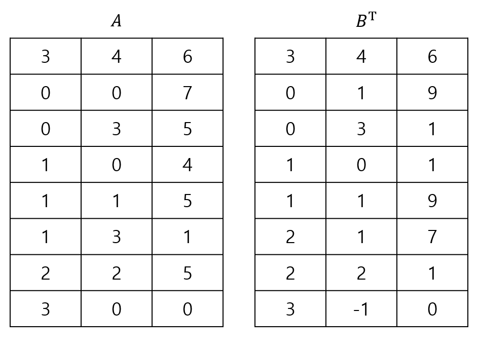
\[A = \begin{pmatrix} 7 & 0 & 0 & 5 \\ 4 & 5 & 0 & 1 \\ 0 & 0 & 5 & 0 \end{pmatrix}, B = \begin{pmatrix} 0 & 1 & 0 \\ 9 & 9 & 7 \\ 0 & 0 & 1 \\ 1 & 0 & 0 \end{pmatrix}\]

먼저 행렬은 희소 행렬을 표현하던 방식과 동일하게 표현한다고 가정합니다. 그럼 $A$와 $B$가 다음과 같이 저장됩니다.

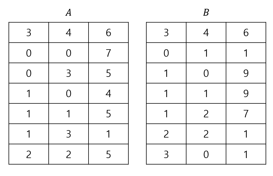
이전에 배운 Fast Transpose를 이용하여 행렬 $B$의 전치 행렬을 구합니다.

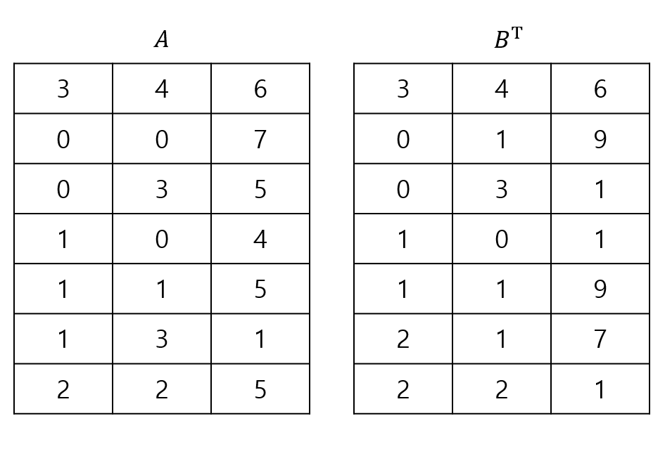
그 다음, 다음과 같이 행렬 $A$의 아래에는 (행의 수, 0, 0)을 삽입하고, 행렬 $B^{\sf T}$의 전치 행렬 아래에는 (열의 수, -1, 0)을 삽입합니다.

이렇게 보시면 어떻게 행렬의 곱셈을 수행해야 할지 대략 감이 오실 것 같습니다. 두 행렬을 위부터 차례대로 내려가면서 행과 열이 같은 경우에만 곱셈을 수행한 다음, 곱셈 결과를 저장할 배열에 삽입하고, 그 외에는 전부 무시하면서 패스하면 되기 때문입니다. 이렇게 행렬의 곱셈을 수행한 결과를 행렬 $D$라고 하면, 결과는 다음과 같이 나오게 됩니다.

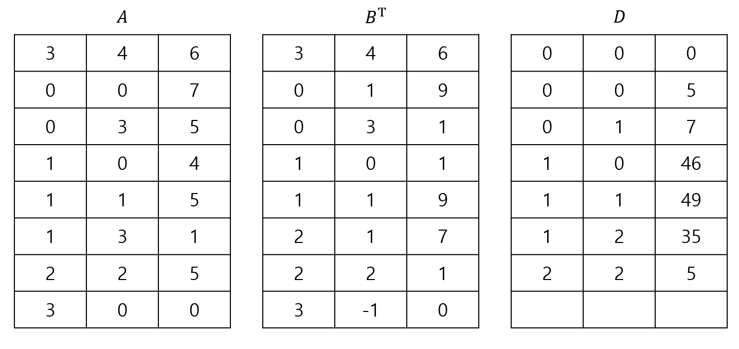
이것을 다시 행렬로 표기하면 다음과 같습니다.

\[\begin{pmatrix} 7 & 0 & 0 & 5 \\ 4 & 5 & 0 & 1 \\ 0 & 0 & 5 & 0 \end{pmatrix} \begin{pmatrix} 0 & 1 & 0 \\ 9 & 9 & 7 \\ 0 & 0 & 1 \\ 1 & 0 & 0 \end{pmatrix} = \begin{pmatrix} 5 & 7 & 0 \\ 46 & 49 & 35 \\ 0 & 0 & 5 \end{pmatrix}\]

이 과정을 그대로 프로그램으로 만들면 다음과 같습니다.

Program 2.10: Sparse matrix multiplication

void mmult(term a[], term b[], term d[])
/* multiply two sparse matrices */
{
	int i, j, column, totalb = b[0].value, totald = 0;
	int rows_a = a[0].row, cols_a = a[0].col, totala = a[0].value;
	int cols_b = b[0].col;
	int row_begin = 1, row = a[1].row, sum = 0;
	term new_b[MAX_TERMS];
	if (cols_a != b[0].row) {
		fprintf(stderr, "Incompatible matrices\n");
		exit(1);
	}
	fast_transpose(b, new_b);
	/* set boundary condition */
	a[totala + 1].row = rows_a;
	new_b[totalb + 1].row = cols_b; new_b[totalb + 1].col = -1;
	for (i = 1; i <= totala; ) {
		column = new_b[1].row;
		for (j = 1; j <= totalb + 1; ) {
			/* multiply row of a by column of b */
			if (a[i].row != row) {
				storeSum(d, &totald, row, column, &sum);
				i = row_begin;
				for (; new_b[j].row == column; j++)
					;
				column = new_b[j].row;
			}
			else if (new_b[j].row != column) {
				storeSum(d, &totald, row, column, &sum);
				i = row_begin;
				column = new_b[j].row;
			}
			else switch (COMPARE(a[i].col, new_b[j].col)) {
			case -1: /* go to next term in a */
				i++; break;
			case 0: /* add terms, go to next term in a and b */
				sum += (a[i++].value * new_b[j++].value);
				break;
			case 1: /* go to next term in b */
				j++;
			}
		} /* end of for j <= totalb+1 */
		for (; a[i].row == row; i++)
			;
		row_begin = i; row = a[i].row;
	} /* end of for i <= totala */
	d[0].row = rows_a; d[0].col = cols_b;
	d[0].value = totald;
}

Program 2.11: storeSum function

void storeSum(term d[], int* totalD, int row, int column, int* sum) {
	/* if *sum != 0, then it along with its row and column
	   position is stored as the *totalD+1 entry in d */
	if (*sum) {
		if (*totalD < MAX_TERMS) {
			d[++*totalD].row = row;
			d[*totalD].col = column;
			d[*totalD].value = *sum;
			*sum = 0;
		}
		else {
			fprintf(stderr, "Numbers of terms in product exceeds %d\n", MAX_TERMS);
			exit(EXIT_FAILURE);
		}
	}
}

먼저, 함수 mmult에서 사용하는 변수에 대해 간략하게 정리해보겠습니다.

• row : 현재 B의 열과 곱하고 있는 A의 행
• row_begin : 현재 행에서 첫 번째 원소의 위치
• column : 현재 A의 행과 곱하고 있는 B의 열
• totald : 행렬의 곱을 저장하는 행렬 D의 현재 원소 갯수
• i, j : A 행과 B 열에서 연속적으로 원소들을 검사하는데 사용함

함수 mmult가 기존에 비해 얼마나 효율적인지 시간 복잡도를 계산해봅시다. for 문을 실행하기 전에 있는 Fast Transpose에서 $O(\text{cols_b} + \text{totalb})$의 시간 복잡도가 소요됩니다. for 문의 시간 복잡도를 계산하는 것은 복잡하기 때문에 하나하나 따져봅시다. 먼저, 바깥쪽 for 문은 totala 만큼 반복됩니다. 이 for 문 안쪽에 for 문이 2개가 있는데, 안쪽의 첫 번째 for 문은 최대 totalb+1만큼 반복됩니다.

그럼 안쪽의 두 번째 for 문이 얼마나 반복하는지 계산해봅시다. 만약 행 $k$의 원소의 수를 $r_k$라고 한다면, i는 최대 $r_k$회만큼 증가됩니다. 그리고 i는 최대 cols_b회만큼 row_begin으로 리셋됩니다. 따라서 두 번째 for 문에서 i의 최대 증가 횟수는 $\text{cols_b} \cdot r_k$회입니다.

즉, 안쪽 for 문들의 시간 복잡도를 계산하면 $O(\text{cols_b} \cdot r_k + \text{totalb})$가 됩니다. 그럼 안쪽 for 문이 행렬 A의 행 수만큼 반복되는 것이기 때문에 다음과 같이 계산할 수 있습니다.

\[\begin{align} \sum_{k=0}^{\text{rows_a}-1} O(\text{cols_b} \cdot r_k + \text{totalb}) &= O(\text{cols_b} \cdot \sum_{k=0}^{\text{rows_a}-1} r_k + \text{rows_a} \cdot totalb) \\ &= O(\text{cols_b} \cdot \text{totala} + \text{rows_a} \cdot \text{totalb}) \end{align}\]

일반적인 경우, $\text{totala} = O(\text{rows_a} \cdot \text{cols_a})$, $\text{totalb} = O(\text{rows_b} \cdot \text{cols_b})$이므로 함수 mmult의 시간 복잡도는 $O(\text{rows_a} \cdot \text{cols_a} \cdot \text{cols_b})$로 나타낼 수 있습니다.

fast_transpose 함수, mmult 함수, storeSum 함수에 main 함수를 포함하여 전체 프로그램을 구현하면 다음과 같습니다.

#include <stdio.h>
#include <stdlib.h>

#define MAX_TERMS 101 /* maximum number of terms + 1 */
#define MAX_COL 50 /* maximum number of column */
#define COMPARE(x, y) (((x) < (y)) ? -1 : ((x) == (y)) ? 0 : 1)

typedef struct {
	int col;
	int row;
	int value;
} term;

void fast_transpose(term a[], term b[]);
void mmult(term a[], term b[], term d[]);
void storeSum(term d[], int* totalD, int row, int column, int* sum);

int main() {
	term a[MAX_TERMS], b[MAX_TERMS], d[MAX_TERMS];
	int end;

	/* set the matrix A */
	a[0].row = 3; a[0].col = 4; a[0].value = 6;
	a[1].row = 0; a[1].col = 0; a[1].value = 7;
	a[2].row = 0; a[2].col = 3; a[2].value = 5;
	a[3].row = 1; a[3].col = 0; a[3].value = 4;
	a[4].row = 1; a[4].col = 1; a[4].value = 5;
	a[5].row = 1; a[5].col = 3; a[5].value = 1;
	a[6].row = 2; a[6].col = 2; a[6].value = 5;

	/* set the matrix B */
	b[0].row = 4; b[0].col = 3; b[0].value = 6;
	b[1].row = 0; b[1].col = 1; b[1].value = 1;
	b[2].row = 1; b[2].col = 0; b[2].value = 9;
	b[3].row = 1; b[3].col = 1; b[3].value = 9;
	b[4].row = 1; b[4].col = 2; b[4].value = 7;
	b[5].row = 2; b[5].col = 2; b[5].value = 1;
	b[6].row = 3; b[6].col = 0; b[6].value = 1;

	/* multiply matrix */
	mmult(a, b, d);

	/* print matrix D */
	for (int i = 0; i <= d[0].value; i++)
		printf("%d %d %d\n", d[i].row, d[i].col, d[i].value);

	return 0;
}

void fast_transpose(term a[], term b[]) 
{ /* the transpose of a is placed in b */
	int row_terms[MAX_COL], starting_pos[MAX_COL];
	int i, j, num_cols = a[0].col, num_terms = a[0].value;
	b[0].row = num_cols; b[0].col = a[0].row;
	b[0].value = num_terms;
	if (num_terms > 0) { /* nonzero matrix */
		for (i = 0; i < num_cols; i++) row_terms[i] = 0;
		for (i = 1; i <= num_terms; i++) row_terms[a[i].col]++;
		starting_pos[0] = 1;
		for (i = 1; i < num_cols; i++)
			starting_pos[i] = starting_pos[i - 1] + row_terms[i - 1];
		for (i = 1; i <= num_terms; i++) {
			j = starting_pos[a[i].col]++;
			b[j].row = a[i].col; b[j].col = a[i].row;
			b[j].value = a[i].value;
		}
	}
}

void mmult(term a[], term b[], term d[])
/* multiply two sparse matrices */
{
	int i, j, column, totalb = b[0].value, totald = 0;
	int rows_a = a[0].row, cols_a = a[0].col, totala = a[0].value;
	int cols_b = b[0].col;
	int row_begin = 1, row = a[1].row, sum = 0;
	term new_b[MAX_TERMS];
	if (cols_a != b[0].row) {
		fprintf(stderr, "Incompatible matrices\n");
		exit(1);
	}
	fast_transpose(b, new_b);
	/* set boundary condition */
	a[totala + 1].row = rows_a;
	new_b[totalb + 1].row = cols_b; new_b[totalb + 1].col = -1;
	for (i = 1; i <= totala; ) {
		column = new_b[1].row;
		for (j = 1; j <= totalb + 1; ) {
			/* multiply row of a by column of b */
			if (a[i].row != row) {
				storeSum(d, &totald, row, column, &sum);
				i = row_begin;
				for (; new_b[j].row == column; j++)
					;
				column = new_b[j].row;
			}
			else if (new_b[j].row != column) {
				storeSum(d, &totald, row, column, &sum);
				i = row_begin;
				column = new_b[j].row;
			}
			else switch (COMPARE(a[i].col, new_b[j].col)) {
			case -1: /* go to next term in a */
				i++; break;
			case 0: /* add terms, go to next term in a and b */
				sum += (a[i++].value * new_b[j++].value);
				break;
			case 1: /* go to next term in b */
				j++;
			}
		} /* end of for j <= totalb+1 */
		for (; a[i].row == row; i++)
			;
		row_begin = i; row = a[i].row;
	} /* end of for i <= totala */
	d[0].row = rows_a; d[0].col = cols_b;
	d[0].value = totald;
}

void storeSum(term d[], int* totalD, int row, int column, int* sum) {
	/* if *sum != 0, then it along with its row and column
	   position is stored as the *totalD+1 entry in d */
	if (*sum) {
		if (*totalD < MAX_TERMS) {
			d[++*totalD].row = row;
			d[*totalD].col = column;
			d[*totalD].value = *sum;
			*sum = 0;
		}
		else {
			fprintf(stderr, "Numbers of terms in product exceeds %d\n", MAX_TERMS);
			exit(EXIT_FAILURE);
		}
	}
}

위의 프로그램에서 main 함수에는 예제와 동일한 행렬 데이터를 삽입했습니다. 실행하시면 동일한 결과가 나온다는 것을 확인하실 수 있습니다.

Representation of Multidimensional Arrays

이번에는 다차원 배열을 표현하는 방법에 대해 알아보겠습니다. 기본적으로 다차원 배열은 $a[upper_0][upper_1] \cdots [upper_{n-1}]$과 같은 형식으로 표현합니다. 이러한 다차원 배열에서 총 원소의 수는 $\prod_{i=0}^{n-1} upper_i$로 간단하게 계산할 수 있습니다.

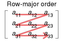
이러한 다차원 배열을 표현할 때는 행을 기준으로 나타낼 것인가(Row major order), 열을 기준으로 나타낼 것인가(Column major order)를 결정해야 합니다.

먼저 행을 기준으로 나타내는 Row major order는 지금까지 저희가 2차원 배열을 나타냈던 방식과 동일합니다. 이해하기 쉽게 그림으로 도식화를 하면 다음과 같습니다.

Row major order에서 주소값을 계산해봅시다. 만약 시작 주소가 $a$라고 가정하고, 2차원 배열이 $a[upper_0][upper_1]$로 정의되었다고 가정하면 $a[i][j]$의 주소는 $a + i \cdot upper_1 + j$가 됩니다. 3차원 배열인 경우 $a[upper_0][upper_1][upper_2]$로 정의되었다고 가정했을 때, $a[i][j][k]$의 주소는 $a + i \cdot upper_1 \cdot upper_2 + j \cdot upper_2 + k$로 나타낼 수 있습니다.

반대로 Column major order는 순서를 계산하는 방식이 조금 다릅니다. Column major order의 접근 순서를 도식화하면 다음과 같습니다.

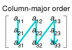
Column major order에서 $a[i][j]$의 주소를 계산하면 $a + j \cdot upper_1 + i$가 됩니다. 간단하죠? 3차원 배열인 경우도 마찬가지로 $a[i][j][k]$의 주소는 $a + k \cdot upper_1 \cdot upper_2 + j \cdot upper_2 + i$로 나타낼 수 있습니다.

프로그래밍 언어마다 다차원 배열에서의 접근 순서는 다릅니다. 기본적으로 C를 비롯한 C-like 언어에서는 Row major order를 사용하지만, MATLAB, R과 같은 언어에서는 Column major order를 사용합니다. 다만 여러분이 자주 사용하실만한 언어는 대부분 Row major order를 사용하기 때문에 이러한 분류가 있다 정도만 알고 계시면 될 것 같습니다.

다음은 2장의 마지막 부분인 문자열(String)에 대해 다뤄보겠습니다. 읽어주셔서 감사합니다!